25.2 Bootstrapping

How can we estimate the variability in a statistic? Let’s say we want a probability interval for the mean of some data.

n = 100
simData = rgamma(n, 2, 1)
# True mean: 2
hist(simData)

mean(simData)
## [1] 2.04451

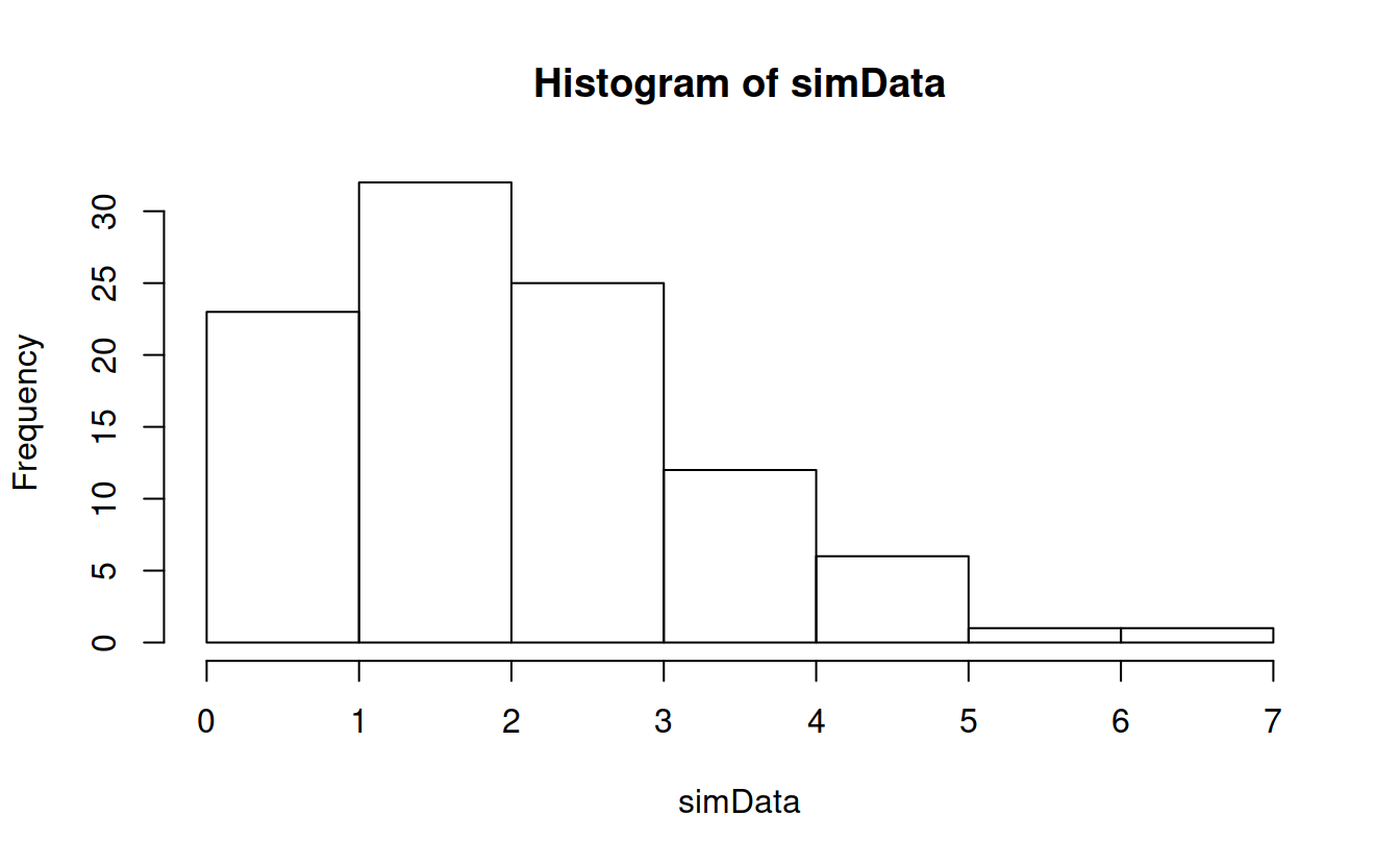
One option is to rely on normal theory and write,

\[var(\bar{x}) = \frac{1}{n}var(x),\] then use the right normal score to get the ``confidence interval’’ you want:

xbar = mean(simData)
xsd = sd(simData)
# 95% interval
confInt = xbar + c(-1.96, 1.96) * (xsd/sqrt(n))
confInt
## [1] 1.800013 2.289007

The accuracy of this estimate depends on the extent to which the data are normal. We know the data are from a rather skewed gamma, how much does that skewness affect the interval? How could we find out?

What if we had some large number of samples, say m, of the mean computed from \(n\) samples of this population? This is an awful idea in practice, but bear with me.

m = 2000
simulatedMeans = numeric(m)
# don't need for loop for this
for (i in 1:m) simulatedMeans[i] = mean(rgamma(n, 2, 1))

quantile(simulatedMeans, c(.025, .975))
##     2.5%    97.5% 
## 1.734263 2.283977

confInt
## [1] 1.800013 2.289007

We can visualize this:

plotSequence = seq(min(simulatedMeans), max(simulatedMeans), length = 1000)
hist(simulatedMeans, prob = TRUE, sub = "Line is the normal approximation density")
lines(plotSequence, dnorm(plotSequence, mean = xbar, sd = xsd/sqrt(n)))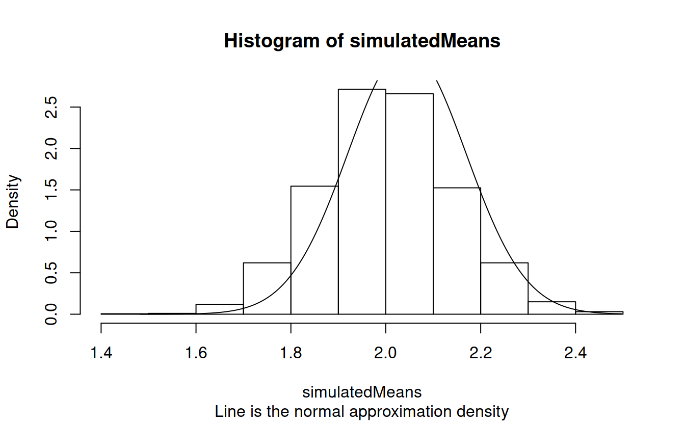

Obviously, we can’t just get a thousand means to estimate its variability, but we can do something close by resampling from our original data. This is called bootstrapping.

# b represents the number of bootstrap samples
b = 2000
bootstrapMeans = numeric(b)
for(i in 1:b){
  resample = sample(simData, n, replace = TRUE)
  bootstrapMeans[i] = mean(resample)
} 

quantile(simulatedMeans, c(.025, .975))
##     2.5%    97.5% 
## 1.734263 2.283977

quantile(bootstrapMeans, c(.025, .975))
##     2.5%    97.5% 
## 1.807087 2.300364

confInt
## [1] 1.800013 2.289007

hist(simulatedMeans, prob = TRUE, sub = "Line is the normal approximation density", col = rgb(1, 0, 0, .2))
hist(bootstrapMeans, prob = TRUE, col = rgb(0, 0, 1, .2), add = TRUE)
lines(plotSequence, dnorm(plotSequence, mean = xbar, sd = xsd/sqrt(n)))
legend("topright", bty = 'n', fill = c("red", "blue"), legend = c("True Mean Dist", "Bootstrap Dist"))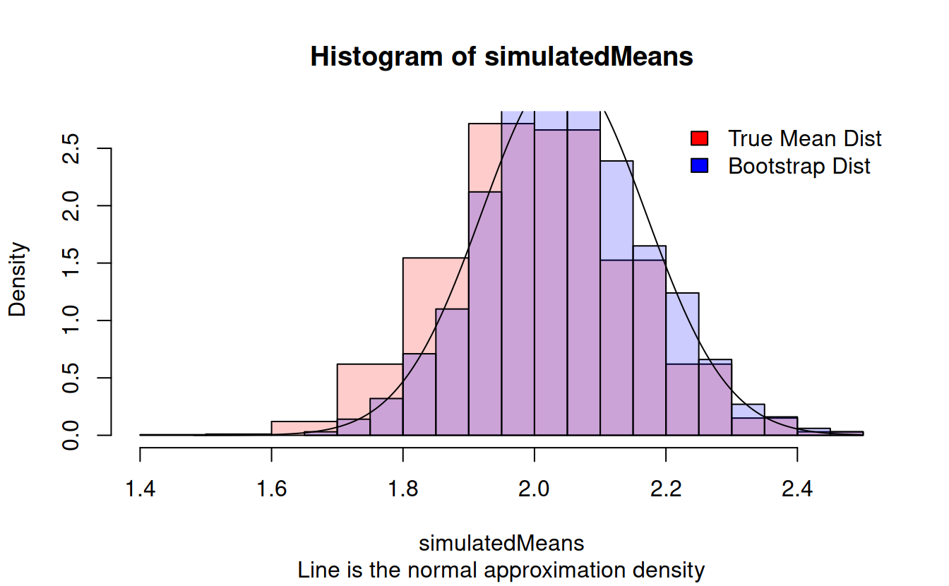

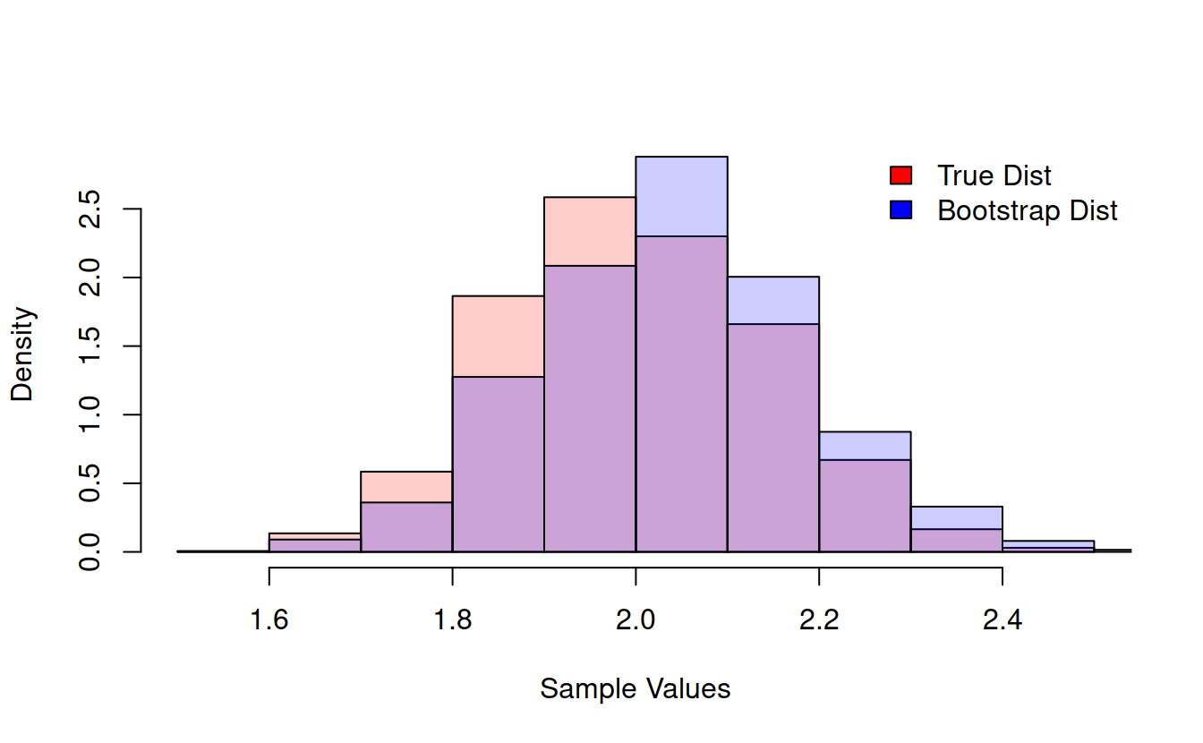
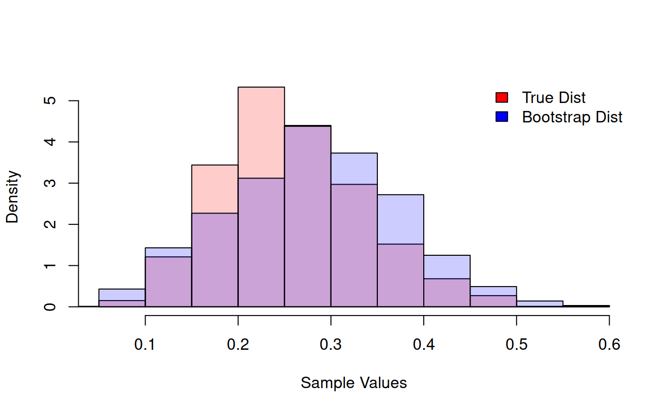
We see that this strange resampling technique seems to work well when we want to find a mean, at least as well as the normal approximation. Its true strength lies in estimating variability in more exotic statistics. For example, what is the variability in the width of the 95% confidence probability interval for our gamma data?

confintWidth = function(data){
  upperAndLowerBounds = quantile(data, c(.025, .095))
  width = diff(upperAndLowerBounds)
  names(width) = NULL
  return(width)
}

confintWidth(simData)
## [1] 0.1734299

m = 2000
simulatedWidths = numeric(m)
for (i in 1:m) simulatedWidths[i] = confintWidth(rgamma(n, 2, 1))

quantile(simulatedWidths, c(.025, .975))
##      2.5%     97.5% 
## 0.1232144 0.4330531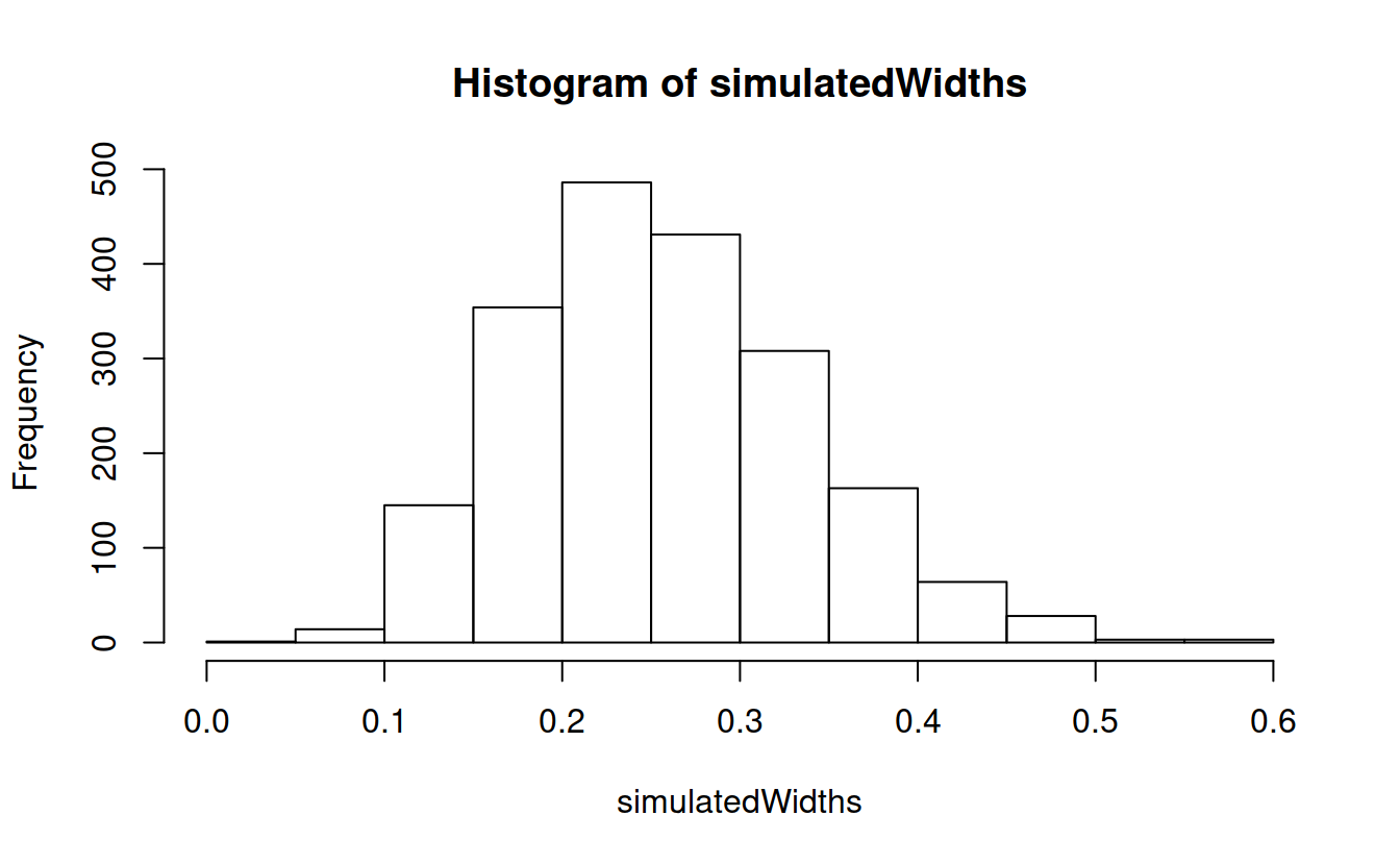

hist(simulatedWidths)

b = 2000
bootstrapWidths = numeric(b)
for(i in 1:b){
  resample = sample(simData, n, replace = TRUE)
  bootstrapWidths[i] = confintWidth(resample)
} 

quantile(simulatedWidths, c(.025, .975))
##      2.5%     97.5% 
## 0.1232144 0.4330531

quantile(bootstrapWidths, c(.025, .975))
##       2.5%      97.5% 
## 0.07638408 0.47030471

hist(simulatedWidths, prob = TRUE, col = rgb(1, 0, 0, .2))
hist(bootstrapWidths, prob = TRUE, col = rgb(0, 0, 1, .2), add = TRUE)
legend("topright", bty = 'n', fill = c("red", "blue"), legend = c("True Mean Dist", "Bootstrap Dist"))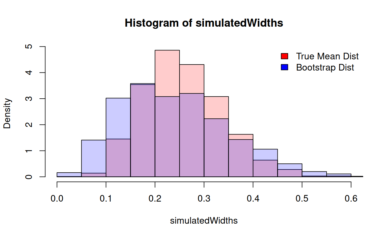

We can do this with any function at all!

compareBootstrapToTruth = function(functionToCompare, sampleSize = 100, resamples = 1000, plot = FALSE, ret = FALSE){
  
  data = rgamma(sampleSize, 2, 1)
  trueSamples = numeric(resamples)
  bootstrapSamples = numeric(resamples)
  if(class(functionToCompare(data)) != "numeric") stop("Function must return a scalar.")
  
  for(i in 1:m){
    trueSamples[i] = functionToCompare(rgamma(sampleSize, 2, 1))
    resample = sample(data, sampleSize, replace = TRUE)
    bootstrapSamples[i] = functionToCompare(resample)
  } 
  
  if(plot){
    trueHist = hist(trueSamples, plot = FALSE)
    bootHist = hist(bootstrapSamples, plot = FALSE)
    hist(trueSamples, prob = TRUE, col = rgb(1, 0, 0, .2), main = "", xlab = "Sample Values", ylim = c(0, max(trueHist$density, bootHist$density)))
    hist(bootstrapSamples, prob = TRUE, col = rgb(0, 0, 1, .2), add = TRUE)
    legend("topright", bty = 'n', fill = c("red", "blue"), legend = c("True Dist", "Bootstrap Dist"))
  }
  out = list(trueSamples = trueSamples, bootstrapSamples = bootstrapSamples)
  if(ret) return(out)
}

compareBootstrapToTruth(mean, plot = TRUE)

compareBootstrapToTruth(confintWidth, plot = TRUE)