5.6 Statistical Transformations

dim(diamonds)
## [1] 53940    10

head(diamonds)
## # A tibble: 6 x 10
##   carat cut       color clarity depth table price     x     y     z
##   <dbl> <ord>     <ord> <ord>   <dbl> <dbl> <int> <dbl> <dbl> <dbl>
## 1 0.23  Ideal     E     SI2      61.5    55   326  3.95  3.98  2.43
## 2 0.21  Premium   E     SI1      59.8    61   326  3.89  3.84  2.31
## 3 0.23  Good      E     VS1      56.9    65   327  4.05  4.07  2.31
## 4 0.290 Premium   I     VS2      62.4    58   334  4.2   4.23  2.63
## 5 0.31  Good      J     SI2      63.3    58   335  4.34  4.35  2.75
## 6 0.24  Very Good J     VVS2     62.8    57   336  3.94  3.96  2.48

ggplot(data = diamonds) + geom_bar(mapping = aes(x = cut))

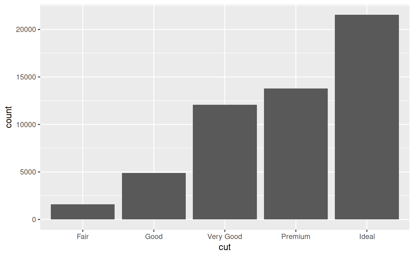
Use a stat to calculate a new value. diamonds data gets “transformed” into a frequency table that get’s plotted by the bar plot.

Look at the geom_bar documentation, you will see the stat will be count (i.e., stat_count()).

ggplot(data = diamonds) + stat_count(mapping = aes(x = cut))

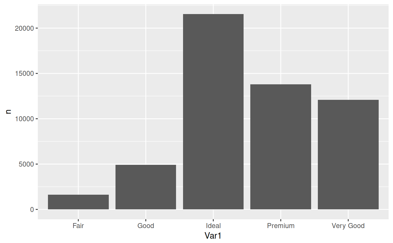
You can set stat to ‘identity’ if you have already calculated a frequency table

pre_counted <- tibble::as.tibble(table(diamonds$cut))

ggplot(data = pre_counted) +
  geom_bar(
    mapping = aes(x = Var1, y = n), stat = 'identity'
  )

# overwrite default stat
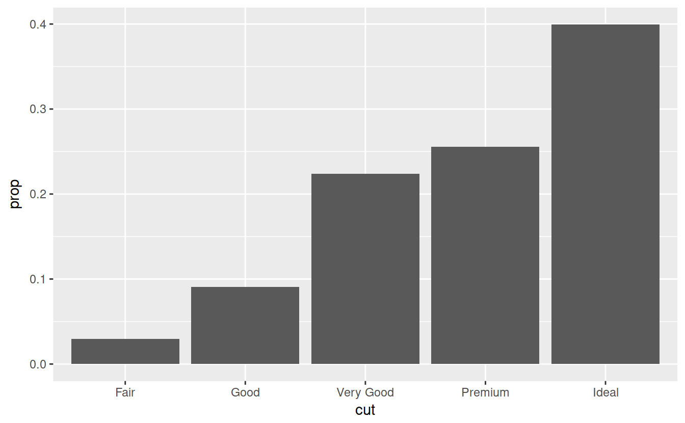
# proportion instead of count
ggplot(data = diamonds) +
  geom_bar(
    mapping = aes(x = cut, y = ..prop.., group = 1)
  )

grouping: http://ggplot2.tidyverse.org/reference/aes_group_order.html

By default, the group is set to the interaction of all discrete variables in the plot. This often partitions the data correctly, but when it does not, or when no discrete variable is used in the plot, you will need to explicitly define the grouping structure, by mapping group to a variable that has a different value for each group.