25.4 Viewing Random Forests
The last part of the course will introduce you to the random forest package, some nifty things you can do with it, and some visuals. IMPORTANT NOTE!!! This implementation of random forest can’t handle catgegorical predictors directly. You need to convert them to a model matrix. This isn’t that hard, but if you’re not aware of it you can get spurious results
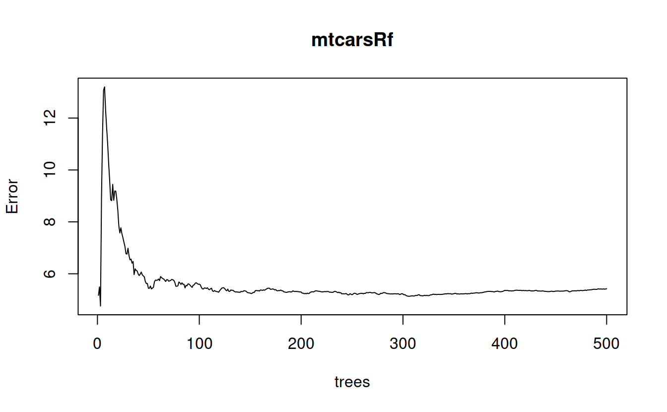
mtcarsRf = randomForest(mpg ~ ., data=mtcars, importance=TRUE, proximity=TRUE, mtry = 4)
mtcarsRf
##
## Call:
##  randomForest(formula = mpg ~ ., data = mtcars, importance = TRUE,      proximity = TRUE, mtry = 4)
##                Type of random forest: regression
##                      Number of trees: 500
## No. of variables tried at each split: 4
##
##           Mean of squared residuals: 5.424577
##                     % Var explained: 84.58
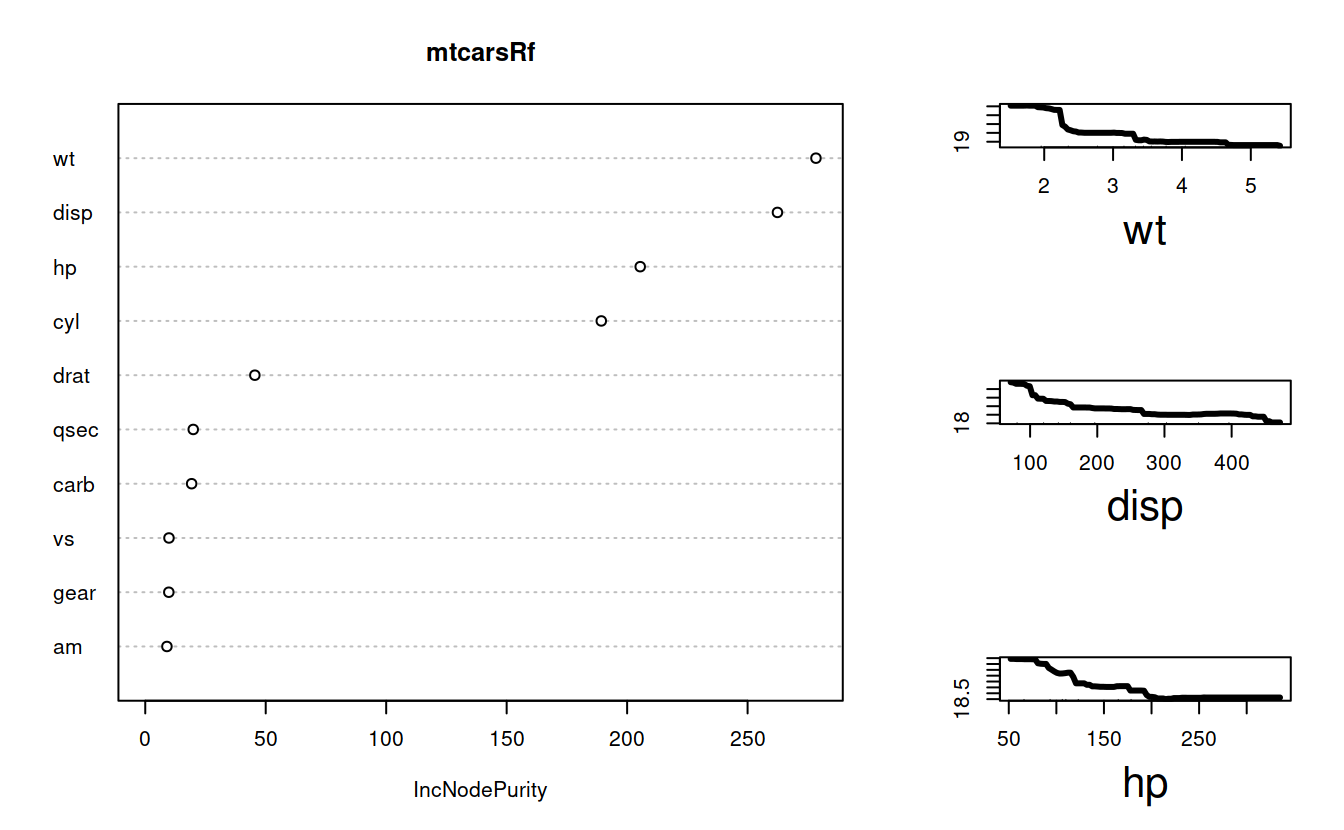
Variable importance.
varImportance = importance(mtcarsRf, type = 2)
varImportance
##      IncNodePurity
## cyl     189.275498
## disp    262.391424
## hp      205.431608
## drat     45.489344
## wt      278.369216
## qsec     19.915649
## vs        9.846512
## am        8.995382
## gear      9.776913
## carb 19.251604layout(matrix(c(1,1,2,1,1,3,1, 1, 4), nrow = 3, ncol = 3, byrow = TRUE))
varImpPlot(mtcarsRf, type = 2)
impvar = rownames(varImportance)[order(varImportance[, 1], decreasing=TRUE)]
colors = c("black", "blue", "red")
for(j in 1:3){
partialPlot(mtcarsRf, mtcars, impvar[j], main = "",xlab = impvar[j], lwd= 3, cex.lab = 2, n.pt = 100)
}
A neat output of an RF model is a measure of proximity between rows. Proximity is the proportion of times two observations appear in the same leaf node. This can be very useful in cases where rows contain both continuous and categorical data, a typically difficult situation for most metrics.
If we do 1 - proximity we can turn this into a distance matrix and do things like multidimensional scaling.